Cosmic Ray Air Shower Array
Here, I describe what I did for the High Energy Group in the LSU Physics Department.
Introduction to the Physics & Hardware
Introduction
I worked in the physics department at LSU for some time, between 1999 and 2002. I worked with the neutrino guys (SuperK and KamLAND) for a bit then was passed on to the cosmic ray people. Right before I left to enter the world as a web developer, I decided to make this presentation to later remind myself what all I did.
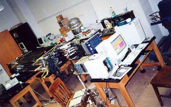
Figure 1a : Early testing and calibrating of phototubes: stack configuration.
I'll begin with Figure 1a. This is a picture of the old cramped room before the Nicholson Hall annex was built. In the foreground to the right you see a PC with KmaxNT, the data acquisition (DAQ) software package, running. To the left of the monitor is a CAMAC minicrate with several hardware modules inside. Behind the grey minicrate is a small NIM bin (appears light blue because of hardware modules in it). Behind the monitor is a blue high voltage (HV) power supply distribution box. The last thing of interest is the stack of scintillators on the table to the left with phototubes pointing out to the right (with small copper base plates where the HV and signal cables are plugged in).
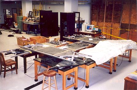
Figure 1b : Final arrangement of counters: array configuration.
In Figure 1b is the air shower array configuration. But more on that later on.
Now, what does all this do? It seems best to start with the phenomenon of cosmic rays.
Cosmetic Ray? What in the Hell Is That Then?
A cosmic ray is a piece of an atom (not a ray, really). There are 2 kinds of particles hitting the Earth's atmosphere:
- galactic cosmic rays − particles from outside the solar system
- solar cosmic rays − obviously, particles from the sun
Figure 2 : A possible air shower.
These particles are bits of atoms, such as H, He, C, O, Fe, Li, Be, and B. To reach the Earth, galactic cosmic rays must go through the solar wind as well as Earth's magnetic field. (More cosmic rays reach the poles than the equator.) The solar wind, though, is less energetic than galactic particles, and so don't penetrate the Earth's magnetic field as much. (A big question is where do really high energy galactic cosmic rays come from. Pulsars? Supernovae?)
So these particles hit atoms in the atmosphere. About 85% are protons (H nucleus), 12% are alpha particles (He nucleus), and 3% are electrons and nuclei of heavier atoms. When these primary incident particles interact with the upper atmosphere, secondary particles are created: protons; neutrons; positive, negative, and neutral pions (mean lifetime of 26ns). Muons (mean lifetime of 2.2μs) and neutrinos are the decay products of charged pions; and electrons, positrons, and gamma rays are the decay products of neutral pions. (Muons decay further into electrons and neutrinos.)
Muons are the largest component of charged cosmic ray particles (because they are so massive -- 207x mass of the electron -- and have a relatively long lifetime). Most muons originate in the upper atmosphere and lose ~2 GeV by the time they reach sea level. The mean energy for muons at sea level is ~4GeV.
Figure 2 shows an example air shower starting with a proton incident on the atmosphere. It hits some atom in the air and splits into a neutron and some pions. The pions decay into muons and so forth. Further, these particles can interact with other atoms in the air and produce more particles.
There's a Muon in My Soup
It is mostly muons that come through down from the sky and through the ceiling. I remember reading that there are 20 muons passing through your body at any one time. That's just what they do. Can't be helped unless you're under a kilometer of rock. To detect these guys, man has created scintillators. I used left-over organic plastic scintillators from some previous experiments. The way these work is the plastic is doped with some kind of atom that gets excited when a muon hits it. As it deexcites, an ultraviolet photon is produced. The trick in producing these scintillators is to have the material transparent to the frequency of photon produced. The photon bounces around and hopefully heads in the direction of the phototube (photomultipler tube, or PMT).
Figure 3 : Muon exciting an atom in the scintillator. The atom
deexcites, producing UV radiation.
Now, it is said that the very best detectors have only a 10% photon collection efficiency. Whatever that means.
So, the muon loses about 2MeV/cm in our scintillator. I guess 10% of that energy goes into the photons that make it to the PMT at the end of the light guide (as Figure 3 shows). The light guide is non-scintillating plastic with an index of refraction close to that of the scintillator.
Photons to Electrons
The photocathode in the PMT must be thick enough to absorb photons but thin enough to prevent absorption of the photoelectrons (produced by the photon striking the photocathode). Photocathodes tend to be Cs-Sb or K-Cs-Sb alloys. The ones I used are 2cm x 2cm and are said to be ~10-30% efficient, although I have no way of really knowing.
Figure 4 : An example of a phototube, showing the dynodes.
About 4-5 electrons are kicked out on each dynode per incident electron. In the end, 105 - 107 electrons per incident photon are created, making a pulse that is >5 mV and ~60 ns long. This pulse gets sent along cable to NIM or CAMAC modules for further use.
PMTs have to be powered since the dynodes need increasing voltages to accelerate the electrons. We have been using 2 types of tubes: those that produce many electrons per photon and those that produce less. This is to get a better idea of the number of particles for an air shower. The difference between the two is that one is higher voltage than the other. Our counters (as they are called) are scintillators with a PMT on each end, so the pair are seeing light from the same particle(s). One side is the low gain (lower voltage and so lower signal for a particle, thus able to see more particles per event before the tube saturates). The other is high gain (higher voltage and so higher signal for a particle: able to see fewer particles for an event before saturation). The ratio we have set right now for high versus low gain is 10:1. Arbitrarily.
The tubes are powered depending on how they perform. The low gains are powered to produce 1 ADC count per particle. (I'll discuss ADC counts and calibration later on.) The high gain are powered to produce 10 counts per particle. The range of voltages used then turns out to be anywhere from 700 to 1100 V.
Determining Events with Triggers
Particles are always streaming down from the sky and not all of them are interesting. We are looking for air showers: those secondary cosmic rays which are produced by a high energy primary particle. There will be more particles per square meter for this type of air shower than the regular old background. These air showers tend to come down in circular cones with the axis more or less being the trajectory of the primary particle.
There are 2 classes of counter used in these experiments: data counters and trigger counters. The data counters are used for data collection. The trigger counters are used to determine when an air shower occurs. You set up trigger counters in some configuration and apply some logic to the signals they produce. If the signals from the triggers meet your criteria for an air shower, you read the data from the data counters. If not, everything is ignored.
Figure 5 : Stack configuration, side view. Pink=trigger. Blue=data.
Figure 6 : Array configuration, top view. Pink=trigger. Blue=data.
We've used two basic configurations. One is the stack (Figure 5): place all data counters on a table like pancakes. Put one trigger counter on the top, one in the middle, and one on the bottom. This configuration is ideal for calibrating the counters as they have the same particles going through them. Triggering in this configuration follows this logic: if all 3 triggers see a particle, take data.
The second configuration is the array (Figure 6). The logic is the same: if all 3 triggers see something, read data. But this configuration is used for detecting larger air showers. The triggers are spaced out and each has to see some number of particles at the same time.
Really, only 2 triggers are needed in either configuration. The array is now being run with only the corner triggers. Three is just a better number for reducing the number of random background noise events.
Trigger Signal Paths
Now to begin introducing the CAMAC and NIM modules. Let's follow what happens to the trigger signals and just how an event is determined to be valid. Figure 7 shows some trigger signal cables going into something called a discriminator and the output of this discriminator going into another discriminator. We set the threshold on the first discriminator to only allow signals greater than some voltage. The greater the threshold voltage, the more energetic particles have to be for them to be considered valid.
What the second discriminator does is set the number of triggers that must be hit at a time, the coincidence. This works because the first discriminator's SUM output has a voltage of the number of input channels over threshold times -50mV. Setting the second discriminator's threshold to -30mV means only 1 trigger must be good (1-fold coincidence). Setting it to -70mV means 2 triggers must be good (2-fold). And so on.
Figure 7 : Signal path for the trigger counters to produce a GATE for the ADC.
The output that we really want from the second discriminator is NIM for the GATE input on the ADC, to tell the ADC whether or not the data counters' signals should be integrated. However, the discriminator only outputs in ECL, so we have to take that ECL and put it through a level translator to convert it into a NIM signal.
Another problem is the ADC GATE should be longer than the signal produced by the second discriminator. (The level translator can't change the signal duration.) We send the level translator's NIM output through a Gate Generator. This resulting NIM signal with certain duration is then used for the ADC's GATE.
Data Signal Paths
Because the trigger signals have to go through so much hardware and the data counters get particle hits at the same time as the trigger counters, the data signals have to be delayed in some way so they can arrive at the ADC within the GATE window to be integrated. This is easy enough: just delay the data signals.
Figure 8 : Signal path for the trigger counters to produce a GATE for the ADC.
Figure 9 : Data signals get integrated during the ADC's GATE window.
This is done with longer cable. We have some delay boxes which are just modules with lots of wire. Each data counter is getting the equivalent of 40 meters of cable before it reaches the ADC. Figure 8 shows all that goes on with the data signal cable.
When the data signals arrive in the ADC input channels, the GATE has already been set and the ADC proceeds to integrate the charges (Figure 9).
If a channel has no signal, only background noise gets integrated. This is known as the pedestal for that ADC channel. A normal pedestal is about 22 ADC counts, or 5.5pC.
CAMAC Crate
The hardware modules discussed above are not stand-alone. The ADC, Discriminator, and Level Translator are placed in slots of a CAMAC crate, a "minicrate" actually as it's only 11 slots instead of the standard 25. Still they are not usable yet. In the two right-most slots of any CAMAC crate is the Crate Controller (CC). This is the module that is the middle-man between the other modules and the computer. Modules talk to the CC and the CC (ours is a SCSI-2 CC) talks to the computer.
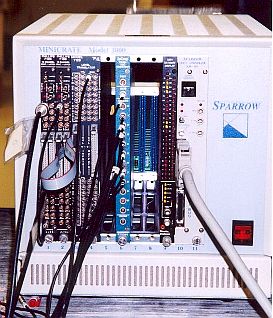
Figure 10 : The minicrate.
The minicrate is shown in Figure 10. In between the blue ADC and the black Dataway Display (with nifty LED lights all over the front) you can see the back, the CAMAC dataway. All modules are plugged in here like Nintendo cartridges so the CC can communicate with them. (Also so they can get power.) The Crate Controller has the SCSI cable plugged into its front.
Some NIM bins are still used for a couple things. The Gate Generator I used was a NIM module as was the Counter, which just counts pulses sent to it. The delay boxes were made with a NIM module shell. (They're just coils of wire.) Also, the HV power supplies are NIM modules. They don't need the NIM bin for power but they have to go somewhere.
That's about it for the hardware and what goes on with the counter signals. Next, I get into the software that is used to read out data and set the thresholds.
Software & Analysis
KmaxNT
Windows 98 is not a real-time operating system so there is no guarantee that a process will execute within a certain time. This is only a problem for runs with a high data rate. For air shower runs where the data rate is only 0.02 Hz or less, this isn't a problem.
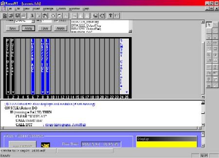
Figure 11 : View of 3 panes.
The software package we use is called KmaxNT, made by Sparrow Corporation. It has a built-in code editor and its own language, Command Sequence Language (CSL). Code is written in one pane of the screen and the user interface is created in another. Things like buttons, progress bars, text fields, and histograms can be created for humans. Widgets like buttons can be tied to specific code blocks (called "events", which is really a procedure, not a data event), so when you click a button called "DoStuff1", the CSL event called "DoStuff1" will be posted to an Event Queue and executed in turn.
Data is written to an "edf" (event data format) file, a peculiar binary format only usable by KmaxNT. Since my data-analyzing world doesn't revolve around KmaxNT, I have written an edf to text converter, named edf2txt. These txt files can be further converted by other programs I've written, such as txt4xl which creates a row of ADC data for each event in the run. This can be easily imported into Excel 2000. (Excel 97 is partial to database queries instead of text files.)
A Typical Event
Before the run is started, a write file (edf file) is opened. Modules are initialized and discriminator thresholds are set. So here's what happens with a normal event:
- A cosmic ray air shower bathes all counters with particles.
- While the data signals get delayed by lengths of cable, the trigger signals get sent to a discriminator.
- For each trigger signal that's greater than the threshold, -50mV are added to a SUM output which gets sent to a second discriminator.
- The second discriminator is set for a certain coincidence of triggers. If the SUM out from the first discriminator is greater than this threshold, an ECL output is sent to a level translator.
- The level translator converts the ECL square wave into a NIM square wave and sends it to a gate generator.
- The gate generator sets the duration of the pulse and sends it to the GATE input of the ADC.
- The ADC receives the GATE window pulse and begins to charge one capacitor for every input channel. When the GATE ends, the capacitors are discharged and the time it takes is converted to a count equivalent to the amount of charge that each input signal contained (0.25pC/count). The values are stored in registers.
- The ADC sends a Look-At-Me (LAM) signal over the CAMAC dataway to the crate controller (CC).
- The CC sends a signal over the SCSI bus to the computer.
- What happens next is cloudy. After an indefinite amount of time (1-170ms), KmaxNT receives the interupt and posts the event "SRQ" to the Event Queue. (SRQ is a predefined procedure in KmaxNT. It exists but you must write the code for what should happen next.)
- I have SRQ checking to see which slot sent the original LAM by asking the CC for its LAM register.
- The CC responds with all slots that presently have a LAM.
- If it was slot 6 (the ADC), I have KmaxNT post a couple events to the Event Queue: "WriteTime" and "ADC_READ".
- "WriteTime" executes when it gets to the front of the Event Queue. It writes the date and time to the open write file.
- When "ADC_READ" gets to the front of the Event Queue, it gets the data from the ADC channels by telling the CC to perform a read operation on slot 6, subaddress 0 through 11. The data is stored in an array. On the last read, the ADC registers are cleared.
- "ADC_READ" then posts another event to the Event Queue which writes the 12 integers to the open write file.
- After the last write to file, the event tells the CC to clear the LAM for slot 6. Things are now ready to repeat.
After the run is over (modules stopped with a toolsheet button I created), the write file is closed.
Analyzing the Data
I've found the quickest way to look at the data is to use Excel 2000. I can import a text file into a template I created and see if the data looks alright. First thing is to run edf2txt on the edf file. I brilliantly have edf2txt run when you click on an edf file. The conversion runs automatically and you're left with a txt file with the same name as the edf. I thought of maybe having the program ask if you also want to run txt4xl, but decided not to because I won't be working there much longer and didn't want to spend the time to code it. So I made txt4xl an option in the menu that comes up when you right-click on a txt file.
So I import the text file that results after the txt4xl conversion, into Excel. One thing to check with the run is that the data is consistent over the entire run, that no tube's gain fluctuated over the run. This would mean some kind of grounding problem in the tube and many further runs to see why. The graph for this is your basic ADC counts versus time.
Next, the pedestals (the background) must be subtracted from each channel's data. (More on how pedestals are determined later.) Another thing to check is that the ratio of high gain tube to low gain tube on each scintillator is 10:1. This is just plotting for each event the high gain data (y) versus low gain (x). The slope should basically be 10 for points in between y=15 and y=400. The reason for stopping at 400 is the ADC can only integrate so much charge and maxes out at 1129 counts. The ratio between high and low is less and less as you move to higher counts, but is fairly consistent for points in said range.
Another important plot is the one where we compare the histograms of like-gain tubes after pedestal subtraction. The shapes for all low gain tubes should look similar as should the high gains.
Looking at these plots, one can determine if voltages need to be changed or if there's a problem with one of the tubes. So everything up to this point is only what to do to calibrate everything. Only now are we finally getting around to real air shower runs. The array is for students, basically. To have them working with cosmic ray detectors. This set-up is to perform runs and compare the data with expected values, in particular air shower energy versus flux. Low energy air showers are frequent and high energy showers are less so. In short, there are equations you can use to calculate the energy of an event (i.e., an air shower) based on the number of particles in the area covered by scintillator. Plot these data and compare to expected values.
Determining Pedestals
I've mentionned the word "pedestal" a lot in reference to the ADC charge integration. Now to finally describe what it is and how to determine it.
If you turn off the PMT (by turning off its HV supply), you get a dead tube. Any integration of the channel associated with this tube during a GATE will give you your background for the channel because there is no signal. (The integration is affected by what cables are connected to the ADC input, so it's best to leave all cables where they normally are during a run.) This background is the minimum amount of charge on the input cable, the pedestal. (The ADC circuit doesn't seem to be able to subtract charge during the GATE, so background charge always adds.)
A pedestal run is when the trigger tubes are powered but the data tubes are not. The thresholds in the discriminators are set to the lowest they can be, -10mV. This is a rate of about 50Hz, the greatest that the PC can do. The bottleneck seems to be Windows since it's not a real-time OS. Otherwise the slow downs would be with KmaxNT's Event Queue. Software is the problem. The old VAX system could only do 3Hz, so this is a vast improvement. Improvements would be using a better OS, using better data acquisition (DAQ) software, using a newer SCSI standard, and getting a faster CC and modules that support Fast-CAMAC. Also, I understand that there's something that has replaced CAMAC though I can't remember what it is.
Epilogue
So that's about it. I have taken you through the entire system and what I did at LSU. The air shower array is set up for student projects. The actual research groups have two set-ups: a scanning table and a test stand. I really never got around to the scanning table. The test stand has drift chambers and I would have liked to work more with that as you can figure out actual paths of the particles. But there has been no push to set it up as it hasn't been touched since 1997.
I leave things in this state and wonder what's to become of all the work I put into it as no one else knows much about the software and the behavior of the modules.